8 VOLATILITY IN TEMPERATURE

In George Bernard Shaw’s play ‘Pygmalion’ that gave rise to the Lerner and Loewe musical ‘My Fair Lady’, Henry Higgins declares that he can tell where a person comes from according to the accent in their speech. Equally, it may be possible to detect the origin of temperature change, natural or otherwise, via a close study of the evolution of temperature over time.

Departures from the 1948-2015 average monthly air temperature are presented below.  The spread on the axes has been adjusted to a common interval of +4 to -4°C to facilitate  comparison.

We are looking for the month that shows the greatest variability over time. We are also interested in the course of temperature change over the entire sixty seven year period.

For economy of effort, we look at two months at a time starting with January and February in the Arctic.

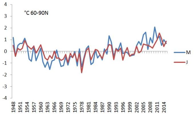
We see that January and February are the months when surface air temperature is most volatile , followed by November and December.

The year to year variation in surface air temperature in January and February is almost as great as the whole of period variation. It is possible that the agent responsible for the inter-annual variation is also responsible for the whole of period variation.  Greenhouse gases that are well mixed never decline from one year to the next. The agent of change on the inter-annual scale produces change in both directions, both positive and negative. Unless we want to throw logic out the window we must look to other modes of causation than the gradual increase in the proportion of well mixed greenhouse gases in the atmosphere for much of and perhaps the entire variation that we observe.

Moreover, the pattern of temperature evolution over time is very different in January and February to the rest of the year. In January and February, the trend is steep and the slope uniform.  In other months, and particularly September and October, temperature falls away in the middle of the period and then rises again. We see also that the difference between beginning and end of the period in September and October is much less than in January and February. There is in fact  very little warming between May and August.

In the same manner we could examine the evolution of temperature by month in the other latitude bands. That would be a slow process.  So, I move directly to show the temperature trace for the particular months where change is most volatile. If you doubt that I have the matter  in hand please check for yourself using the data here: http://www.esrl.noaa.gov/psd/cgi-bin/data/timeseries/timeseries1.pl

We work systematically southwards from the Arctic to the Antarctic. Again, the scales on the following graphs are standardized so as to facilitate comparison between latitude bands. The following are the months when temperature is most volatile.

It is plain that variability falls away with distance from the poles. However least variability is experienced not in the tropics but at 30-60° south latitude. Extreme variability is consistently time specific. January and February are the months of highest variability from the Arctic to 30° south latitude.  The mid and high latitudes of the southern hemisphere  experience strongest variability in July and August.

The time signature for temperature variability suggests an Arctic origin over the bulk of the globe and an Antarctic origin southwards of 30° south latitude. In general, in most interdependent systems the largest disturbances are found close to the source of those disturbances.

WHAT’S HAPPENING?

When I was young I played golf and drank beer. The golf course was frequented by kangaroos. Males kangaroos are apt to fight. Kangaroos grazed the grass in front of the tees and generally led a charmed life with golf balls harmlessly curving through the air overhead. But on one particular occasion a wayward ball skipped across the ground and a male kangaroo took a hit. Instantly he turned and ‘biffed’ his mate. We humans leaned on our clubs and rolled around laughing.

In the normal course of events one can look for the origin of an impact and it will be close by. The kangaroos response was based on observation of the frequency at which blows are received from ones rivals by comparison with the rate at which other forms of misadventure disturbed his life. The energetic ‘biffing’ response was based on experience. The retribution was delivered while the sting of the blow was still fresh.

The extreme variability seen in surface temperature  in mid winter closest to the poles is most likely a response to polar atmospheric processes, not ENSO and definitely not a reaction to the flutter of a butterfly’s wing in the deepest Amazon. So, how does it work?

It is established knowledge that the phenomenon known as the ‘annular modes’ represent the major mode of climate variation that is observed in the atmosphere of the Earth. This annular mode phenomenon involves an interchange of atmospheric mass between latitudes pole-wards of 50° (mostly in winter) and the rest of the globe.  What is not yet appreciated is that the transfer of atmospheric mass is tied to the relative intensity of polar cyclones driven by the ozone content of the atmospheric column above 500 hPa in high latitudes.

Many people are unaware of the enhancement of ozone partial pressure in high latitudes in winter.  To catch up study of the column climatologies here:  http://ds.data.jma.go.jp/gmd/jra/jra25_atlas/eng/indexe_column1.htm

If you don’t go to the JRA 25 Atlas to look at the annual cycle on ozone partial pressure in high latitudes much of what follows may be incomprehensible.

It is very likely that the increase in the length of the atmospheric path taken by short wave radiation of the particular wave lengths that destroy ozone so depletes the wave lengths responsible for that depletion that ozone partial pressure naturally increases with latitude and more particularly so in the winter hemisphere in the vicinity of the polar night zone. In any event the increase occurs. It is these same wave lengths that reach the surface in  damaging intensity when ozone partial pressure is insufficient as it is throughout the entire southern hemisphere by comparison with the northern hemisphere. Here I am referring to the UV Index that increases in summer, and particularly so in the southern hemisphere.

VARIATIONS IN OZONE PARTIAL PRESSURE IN HIGH LATITUDES IN WINTER

Ozone partial pressure varies in that annular ring of high ozone content air that develops between about 55 and 70° of latitude in both hemispheres. I call it the ‘donut’.In describing the manner of its variation I will no doubt dismay and disgust many people who are happy with current modes of thinking about the stratosphere, people who believe that the stratosphere is  a relatively static medium little prone to convection and is not at all influenced by mixing processes of the sort that we see in the troposphere. These people may believe that the major mode of variation in the ozone content of the stratosphere is perhaps via the flux in UV radiation from the sun or perhaps the the uplift of water vapour from the troposphere, planetary waves that arise from the surface……or perhaps even the butterfly in the Amazon. In fact that variation is due to the variable rate of flow of NOx rich air from the mesosphere initiated by the solar wind and greatly amplified by natural atmospheric processes that are probably  common to all planets having nitrogen, oxygen and ozone in their atmosphere.

THE ENERGETIC MEDIUM THAT IS THE STRATOSPHERE

As Gordon Dobson observed, total column ozone maps surface pressure. On the margin of the Antarctic continent in winter there is a well developed ring of ozone rich air (the donut) surrounding a core of ozone deficient air (the hole in the donut), especially prominent in winter. In the Arctic the donut tends to be poorly formed  and very lopsided due to the distribution of land and sea and the dominance of the Pacific Ocean as the major stretch of water that is contiguous to the Arctic. The donut  drives the density of the air and circulation of the entire atmospheric column in high latitudes with particular impact above 500 hPa or five kilometres in elevation. See chapter 4 on the geography of the stratosphere and chapter 5 on the origin of polar cyclones.

The easiest way to see this process in action is to observe the flux in the ozone content of the air in high latitudes at this site:  http://www.cpc.ncep.noaa.gov/products/stratosphere/strat_a_f/

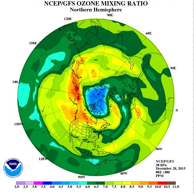
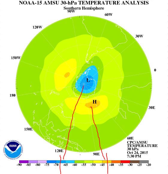
On December 26th 2015, in terms of total column ozone (measured in Dobson units)  as  seen by satellites viewing the Arctic from above we had:

We see ozone poor mesospheric air escaping the very loose containment of an annular ring of ozone rich air (the donut) that is anchored to the endemically low pressure area (rich in ozone) located over the north Pacific. The result is a warming of the polar cap as the warmer ozone rich air on the perimeter migrates inwards and the coldest air migrates outwards leaving only warmer air behind. This is documented below as a sudden stratospheric warming of the type commonly experienced in the Arctic between November and April.

As warmings go this has been brief. We see that the Arctic stratosphere had recently been at the cooler end of the post 1979 range for some months. A warming event manifested about day 357 and peaked on day 360 (December 26th).

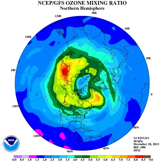
See below: By December 28th the tongue of mesospheric air is reasserting its presence inside the vortex as the annular ring of ozone rich air closes the gate through which the mesospheric air escaped. By the 28th the air in the core has marginally less very ozone deficient air (less deep blue) than before and is accordingly warmer. The escaped mesospheric air has already dissolved into the background as it erodes ozone on the periphery of the ozone rich annular ring on the margins of the polar cap. But there are masses of relatively ozone deficient air at lower latitudes, evidence that the horse has bolted on more than one occasion.

At 10 hPa (30 kilometres) on the 26th December ozone partial pressure looked like this:

By the 28th (as seen below) there is a depression of ozone partial pressure in the cell like structure on the left  where the mesospheric air has been sucked into a column of rising air. The central core that is located over the Arctic is somewhat depleted of its ozone deficient (deep blue) content.

Now look below. On the 26th December the circulation of the atmosphere at 10 hPa shows upward convection of slightly warmer air over the Pacific and descent in the core. Another zone of ascent is seen over the south Atlantic near Africa.

By the 28th (below) the vortex of cold descending air from the mesosphere is intensified and more centred over the Arctic while the temperature of the cell of rising air at 9 o’clock is lower reflecting the absorption of the much colder  mesospheric air that has taken place in that cell of ozone rich rising air. Another cell of rising, relatively warm, ozone rich air  emerges over the Tibetan plateau. The temperature of the mesospheric air in the core is unchanged, as one would expect. These are spot temperatures taken as close as possible to the core of each circulation.

Now, lets transfer our attention to the diagram below. At 30 hPa (23 km) on the 26th of December the donut is much better developed with high ozone values over northern Canada stretching across the North Pacific through to the Eastern Mediterranean.But there is plainly an escape of mesospheric air in process from the cold, ozone deficient polar cap region at five o’clock.

By the 28th (below) the gate is closing and the tongue of mesospheric air is reasserting its presence over the polar cap region. Parcels of relatively ozone deficient air, evidence of previous outflows of mesospheric air circulate in near equatorial latitudes, evidence of vigorous lateral movement on short time scales at this pressure level:

Now we transfer our attention to the figure below representing ozone at 50 hpa (20km). The escape dynamics are consistent with those at 30 hPa (23 km) and 10 hPa (30km) as observed above. 

On the 26th the gate opens and on the 28th it closes:

Plainly, despite a twist in the column, there is continuity of interaction and process between 10 hPa and 50 hPa, over a vertical interval of about 10 km in the heart of what is described, for the want of a better term as the ‘lower stratosphere’.

The thing to note is that it is the flow of ozone deficient mesospheric air through, within (vertically) and beyond the donut that governs the ozone content and the temperature of the air across the hemisphere. We are looking at the beating heart of the polar atmosphere that regulates the flow of erosive mesospheric air into the wider stratosphere. Unlike the human heart that pumps oxygen rich plasma to sustain life, the polar heart pumps a plasma that represents death to ozone in the stratosphere. If the flow of mesospheric air is sustained it will reduce ozone partial pressure, inhibit the formation of polar cyclones and allow atmospheric mass to return to high latitudes. Polar surface atmospheric pressure increases driving very cold air into the mid and low latitudes. Geopotential height falls away in the mid latitudes along with surface pressure and cloud albedo increases. The globe cools.

WHY IS THERE SO LITTLE VARIABILITY IN THE SUMMER STRATOSPHERE?

Lets consider the case of the Antarctic. In late October there is a central core of cold mesospheric air inside the Antarctic vortex as we see below.

By November 6th the core of mesospheric air is slipping away into the wider atmosphere, its rate of replacement so slow as to allow the polar atmosphere to warm to the point where the temperature differential between the core and the donut falls away. The pressure of short wave ionising radiation that destroys ozone increases due to the ever shortening atmospheric path through which that radiation must travel as the sun rises higher in the sky. As ozone partial pressure falls away in the donut and also lower latitudes, the entire southern hemisphere begins to suffer from enhanced levels of damaging ultraviolet light that is a danger to plants and animals.

By December 10th the warmest air lies directly over the  Antarctic continent reversing the  temperature gradient  that existed in October.

THE EVOLUTION OF SURFACE PRESSURE AND WIND OVER ANTARCTICA

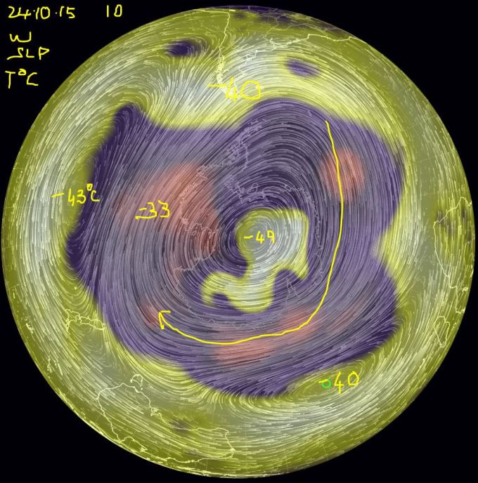
At 10hPa on the 24th Oct the circulation has a core temperature at 10 hPa of -49°C. There is a healthy tongue of mesospheric air situated over the most southerly continent and the circulation is clockwise. Air descends in the core and rises in the low pressure donut.

By 6th November the core temperature at 10hPa has risen to -33°C. The intake of mesospheric air is diminishing.

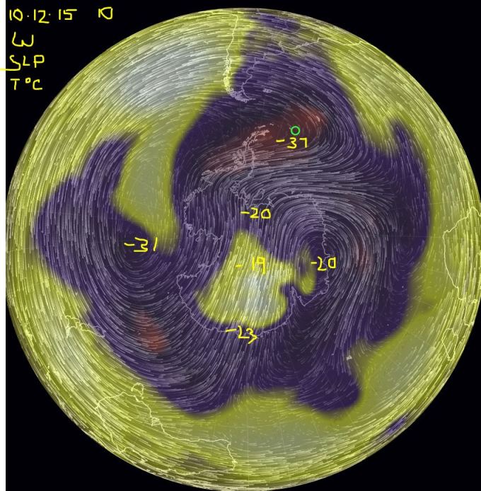
By the 10th December (below) core temperature has risen to -20°C. Ozone partial pressure has fallen away in the donut. the intensity of polar cyclones is  therefore depleted. With that, the vorticity of the overturning circulation that involves a rising donut and a falling core has fallen away. Accordingly the flow of mesospheric air is curtailed and the temperature of the stratosphere no longer fluctuates. There can be little in the way of atmospheric shifts from high to low latitudes if the polar cyclones are starved of the energy that directly reduces atmospheric density in the donut.

By 30th December (below) there is little differentiation in the temperature of low and high latitudes, a core of warm air has set up over Antarctica, the air ascends slowly and the entire circulation is now anticlockwise. The warmest air at 10 hPa is directly over the pole and surface atmospheric pressure falls to its annual minimum. There is no high pressure zone over the Antarctic continent.  Accordingly there can be little variation in the ozone content of the donut in summer. This is the reason why the most extreme surface temperature variation is date stamped either ARCTIC -January-February  or ANTARCTIC- July -August.

CONCLUSION

‘Climate science’ as reflected in the works of the IPCC has no explanation to offer for the interchange of atmospheric mass between high and mid latitudes or the surface temperature swings that are associated with it. Over the Antarctic, as the atmosphere warmed in winter between 1948 and 1978, with peak warming in October, surface pressure fell and has continued to fall, due to ozone enhancement in the donut until recently. Change in the temperature of the globe in all latitudes is intimately associated with this process. I repeat, the IPCC has no explanation for this process. If they did, logic would demand that the AGW thesis would be abandoned.

An uplift that engages the entire atmospheric column of the high latitudes in winter must be balanced by the descent of air from the stratosphere into the troposphere where geopotential heights increase and cloud cover falls away. This increases the amount of solar radiation that reaches the surface of the Earth.  This phenomenon is well observed in that geopotential height increases as surface pressure increases and with it surface temperature but not at all understood. If it were understood the discipline of meteorology could be informed by an understanding of the forces involved rather than having to depend upon rules of thumb based on scattered observation of all sorts of apparently unrelated phenomena. We could then attempt to incorporate the drivers of surface climate in mathematical models on the basis of cause and effect rather than a study of fluid dynamics that takes no cognizance of the fact that we are here dealing with an ‘open system’ subject to influences from the upper atmosphere where the movement of different parcels of air, photolysis and chemical interaction determines atmospheric composition and gives rise to structure.

Climate science is currently built on the assumption that we are dealing with a closed system with all change originating at the surface. It behaves like the male kangaroo that took the impact of the golf ball. If the kangaroo had closely examined the dent in his hide he may have reached a different conclusion as to the cause of the injury. If the I.P.C.C. had a closer look at climate processes it to might change its collective mind and revise its ‘summary for policy makers’. But that wont happen because the science simply does not matter.

If we want to understand climate change we need to come to grips with the processes that are responsible for the change in the partial pressure of ozone in the polar atmosphere. This is the parameter that drives surface pressure, the planetary winds, cloud cover and surface temperature.  We will see that ozone levels climb to a peak in the polar atmosphere in spring but to a variable extent between the years and across the decades. We will see that this process is independent of man’s activities. Furthermore, it is a sufficient explanation of the change in surface temperature that has occurred. But this is a long story that is rich in evidence and will take time in the telling.

The basic parameters of the climate system are forever changing in a fashion that precludes effective modelling, unless we properly apprehend the forces involved.