This chapter explores the characteristics of the atmosphere in spring. It relates the distribution of ozone and NOx to ozonesonde data and the temperature and movement of the air. My data sources are here for maps showing ozone and NOx profiles and here for ozonesonde data and here for maps showing temperature, pressure and wind.
The objective is to investigate the factors responsible for the composition, temperature, density and movement of the air. The discussion pertains to the origin of the planetary winds, cloud cover and surface temperature, in short climate change.

Above: Ozone at 50 hPa 11th to 13th September at six hourly intervals.
The diagrams above show ozone at the 50 hPa pressure level (20km) in the southern hemisphere at 6 hourly intervals. Observe that the rotation of the atmosphere above the Antarctic continent over 54 hours amounts to about half a circle. A full rotation at this rate would take 4.5 days.
It takes about 10 days for a mid latitude anticyclone to pass a point on the Earth’s surface at the latitude of southern Australia. It takes about five days for a polar cyclone to pass from one side of the continent to the other.
As the Earth spins on its axis the morning sun appears on the eastern horizon. The atmosphere moves from the west to the east rotating faster than the Earth itself. The rate of rotation of the atmosphere increases with latitude. In winter, in high latitudes, the rate of rotation also increases with height. This is counter-intuitive. It is commonly asserted that the heat that is absorbed in the tropics is providing the energy to drive the circulation of the air. In general, wherever energy is applied to a system, that is where the most vigorous response is to be found. The movement of the atmosphere, more exaggerated at the poles than at the equator, suggests that the force driving the circulation is being applied at or near the poles. In fact, the greatest depression of surface pressure and the greatest peak in atmospheric pressure on a global scale is to be found in the region of the Antarctic continent in winter. The strongest winds at the surface of the planet merge at 60-70° south latitude. The variation in the temperature of the Earth at every particular latitude is greatest in the middle of winter when the flux in the ozone content of the air is most extreme.
The distribution of ozone at 50 hPa might be described as annular or ring like in shape surrounding the pole. Tracers of ozone fan out towards low latitudes from nodes of relatively high ozone partial pressure. Such a node is located between Antarctica and Australia/New Zealand as seen in the diagram above.
The tracer pattern of ozone distribution is similar to what we observe when a broad bladed paddle is applied to a can of paint. As we stir, a vortex is created in the middle where the centre of the circulation is depressed in relation to the perimeter. Intuitively, the Antarctic circulation is driven in a similar fashion. There is obviously no broad bladed paddle at work. The differences in air density on either side of latitude 60-70° south that give rise to polar cyclones increase as the ozone content of the air is enhanced in winter. The seasonal descent of very cold mesospheric air over the pole chills the interior as the ozone content of the air increases outside the margins of that very cold mesospheric air. These developments together create a situation of atmospheric stress related to extreme differences in air density that is entirely local in origin. We know that the ‘zonal wind’ (east west) varies in conformity with geomagnetic activity. So it is likely that the driving force of this system is in part compositional (density related) and in part electromagnetic in origin.
This description of the forces responsible for the winds in high latitudes is very different to that given in the ‘climate science’ of this day. In fact climate science can not enlighten us as to the origins of the zone of extremely low surface pressure on the margins of Antarctica or the indeed the historical decline in surface pressure in high latitudes let alone the reversal in that process of decline that is currently under-way.None of these features rate a mention. Climate science is dominated by radiative theory and the notion that back radiation from ‘radiation absorbers’ like CO2 and water vapour drives surface temperature. Geographers are out of fashion. Mathematicians and Physicists who know little of the geography of climate hold sway.

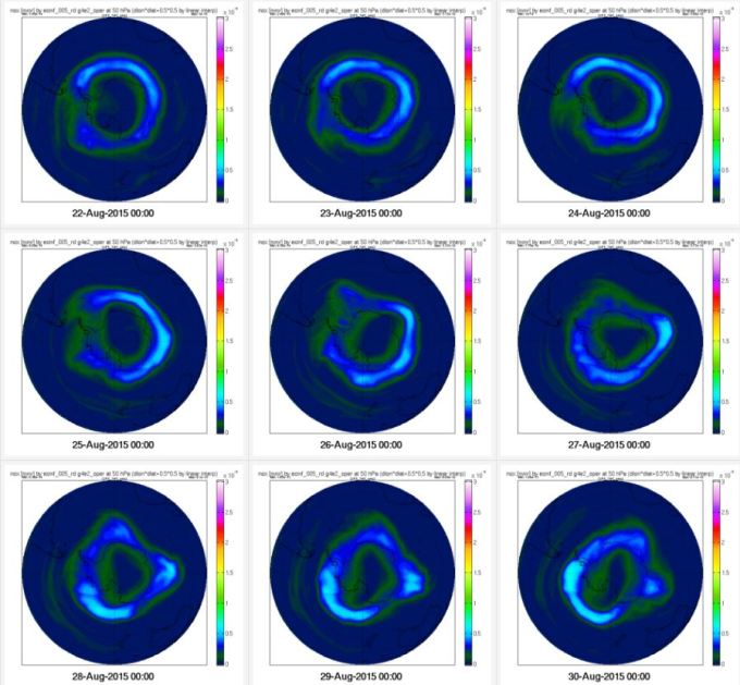
Above: Ozone at 50 hPa at daily intervals.
The diagrams above show the state of the atmosphere at daily intervals. Every particular feature changes in shape over the 24 hour interval between one diagram and the next. There are locations centred on latitude 30° south where ozone partial pressure is low and atmospheric pressure tends to be persistently high. One such lies in the Indian Ocean to the west of Australia a second in the Pacific to the west of the South American continent. A third is located in the South Atlantic to the west of Africa
We can relate the distribution of ozone to that of the chemical family referred to as NOx as seen below. This family catalytically destroys ozone at any temperature. Like any reaction the higher the temperature the faster it will proceed. A catalyst is a substance that increases the rate of a chemical reaction without itself undergoing any permanent chemical change.
Above: NOx at 50 hPa
The NOx that manifests in this ring like fashion originates in the troposphere and enters the Antarctic circulation from the north in a lateral fsashion. See the charts of NOx at 100 hPa below that indicates little or no NOx in high latitudes at this level. There is NOx in low latitudes but none near the poles.
The core of low NOx values at 50 hPa seen above contracts in diameter like the aperture of a camera over the ten days prior to August 30th. As it does so, day by day ozone is eroded.

Above: Nox at 100 hPa.
The distribution of NOx at 50 hPa on the 30th August can be compared to the distribution of ozone and the position of both in relation to the the zone of very low surface pressure that surrounds Antarctica.

I have traced the main features of the distribution of NOx in the diagram above and applied the resulting figure as an overlay on the figure below. NOx manifests in greatest concentration inside the annular ring of ozone rich air. That is as expected, given the ability of NOx to catalytically destroy ozone. The distribution of ozone is therefore a product of the movement of the air and is modulated by the presence or absence of NOx
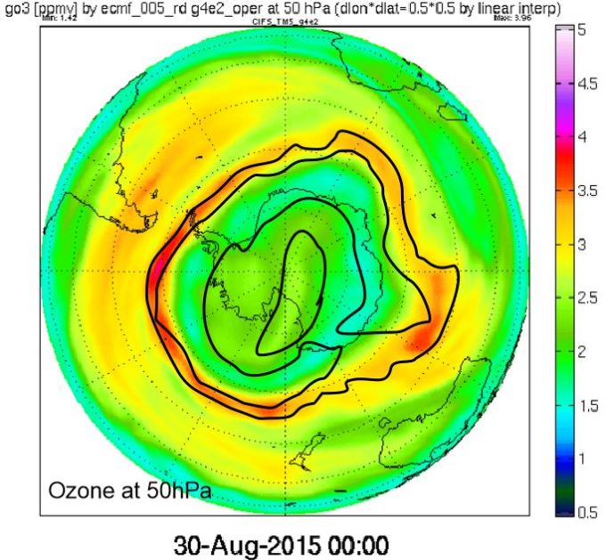
In the same fashion, the figure indicating the distribution of NOx is overlaid on the map of surface pressure and wind at 250 hPa that is below. It is apparent that NOx is drawn into the ascending circulation created by polar cyclones. Air enters the circulation horizontally above 100 hPa and this air shows high concentrations of NOx and very little ozone. In the process it progressively floods the entire area over the Antarctic continent at the 50 hPa level. NOx closes in on the pole like the aperture of a camera. Bear in mind that the distance between the surface where pressure is measured and the 50 hPa level is 20 kilometres. At the surface the distribution of surface pressure is somewhat irregular. At altitude the circulation becomes increasingly smooth and ring like. This is the character of what is called the polar vortex. The vortex does not respect our notions of what is troposphere and stratosphere. It is not particular at all.

An ozonesonde consists of a small piston pump that bubbles ambient air into a cell containing 3 milliliters of 1% potassium iodide solution. The reaction of ozone and iodide produces a small electrical current in the cell, which is proportional to the amount of ozone. The ozonesonde is also interfaced with a radiosonde, which measures air temperature, pressure, relative humidity and transmits all of the data back to a ground receiving station. Total column ozone is calculated by integrating the ozone partial pressure profile up to the balloon burst altitude and adding a residual amount, based on climatological ozone tables, to account for ozone above the balloon burst altitude.
The ozonesonde data below was gathered at the US Amundsen Scott base at the south pole. The distribution of ozone in the diagrams below left relates to the 50 hPa level. Both diagrams relate to the 20th August 2015. Together they give us information about a vertical and a horizontal slice of the atmosphere.
AUGUST: On 26th August the partial pressure of ozone at 50 hPa at the pole is unaffected by the gradual ingress of NOx that is already in evidence on the 7th June at left because it begins only at the outer margins of the continent. The pole is as yet unaffected.

Above: Nox at 50 hPa. NOx occupies more and more of the space over the polar cap from June through to August. The seeds of the ozone hole are planted early. But on the 26th August the polar region is still NOx free.

KEY to diagram on the right: Fine black line: ozone on 26th August (see above). Green line: Generic indicator of pre-ozone hole extent, origin unknown. Blue line: Ozone partial pressure as measured 12 September. Red line: Temperature as measured on 12th September. Fine purple line: Temperature as measured on 26th August.
SEPTEMBER: By 12th September NOx is certainly beginning to erode the partial pressure of ozone over the pole but the extent of erosion depends not on the local temperature (-85°C at 70hPa) or the presence of sunlight (none), or the presence of noctilucent clouds, even though all may be favourable to chlorine chemistry but simply according to the patterns of movement in the air that progressively floods the polar cap with NOx. There are different air masses over the pole, different in their trace gas composition according to the presence or absence of NOx and this is the determining influence so far as total column ozone is concerned.
Notice that the seasonal minimum in total column ozone at the pole manifests between 50 and 100 hPa. There is a marked contrast between this deficit and the high ozone content of the air on the outside of the chain of polar cyclones. The formation of the hole exaggerates the contrast.
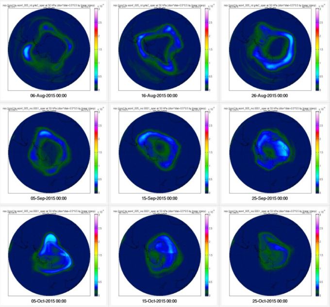
We see below that between 12th September and 15th October NOx floods the polar cap between 100 hPa and 50 hPa and the ozone simply disappears. The outer perimeter of the chain of polar cyclones marks an abrupt transition between high ozone values and virtually none at all. This is the month when surface pressure falls to its annual minimum at 60-70° south. This is not a coincidence. Surface pressure is a function of the vorticity of polar cyclones in turn a function of differences in air density between the northern and southern perimeter of this chain of polar cyclones. With zero ozone on one side of the vortex and a variable amount of ozone on the other side the stage is set for variability that arises entirely according to change in the partial pressure of ozone.
The polar circulation is now changing quickly as the stratosphere undergoes its final warming. See below. There is a strong increase in the temperature of the air above 50 hPa between mid September and mid October.
Notice the warmer air above 25km. Over the polar cap there is insufficient ozone in the air and insufficient air density to allow ozone to make a strong contribution to the temperature of the air above about 25 km in elevation. The increase in the temperature of the air that we observe in this month reflects a reduced influx of very cold mesospheric air and is due entirely to atmospheric dynamics. Warmer air from lower latitudes begins to occupy the polar cap as the polar vortex contracts in diameter and its degree of penetration. The two are actively mixed in the rapidly rotating cross currents of cold descending and warm ascending air across the polar vortex. As we will see the very cold air from the mesosphere enters laterally rather than vertically.
OCTOBER: A reminder: Surface pressure at 60° to 70° south falls to its annual minimum in October when the contrast between the ozone content of the ‘hole’ and its margins is greatest. There should be no doubt as to the motive forces behind this circulation and it has nothing to do with heating in the tropics or any of the circuitous arguments of those who theorise in the world of fluid dynamics who assume that all atmospheric motions can ultimately be put down to heating at the equator and the movements of air masses on a spinning circular orb. A pennyworth of observation is more valuable than a pounds worth of theory.
Below we see that 15th October marks the climax in terms of the presence of NOx over the continent. Unfortunately there is no data for NOx after the 25th November and we have to rely on the distribution of ozone as the sole indicator of the air flow. This is no real hardship because we know that one is always the mirror image of the other. Notice however that NOx declines in concentration after 15th October.
Above: NOx at 50 hPa.
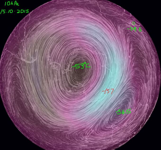
Between the 15th October and the 18th November the air over the pole warms strongly as we see below and the vortex of cold air that descended over the pole is no more. The air in the core of the circulation has a temperature of -53°C on 10th October, and is surrounded by warmer air that is at -15.7°C at its warmest with much colder air on the perimeter and the core of the circulation ends up at -17°C a month later. The air outside the vortex remains at the same temperature.

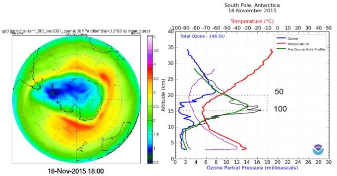
NOVEMBER: The increase in the temperature of the air at 10 hPa (30 km) is reflected in the ozonesonde data for the 18th November. Total column ozone has increased but there is still a marked deficit between 100 hPa and 50 hPa that would be described as an ‘ozone hole’. This deficit can not be accounted for in terms of chlorine chemistry because the air at 50 hPa is now too warm for this to occur. The distribution of ozone simply reflects circulatory phenomena. The diagram at left shows that the greatest deficit in ozone is not above the pole but in the core of the now wandering circulation of swiftly warming air that is no longer locked into its winter position over the pole. 
DECEMBER: It is plain from the diagram at left that the presence or absence of ozone is a product of the movement of the air masses. The ozonesonde data shows that at the 100 hPa level ozone is still heavily depleted by comparison with the August pattern indicating that disparate winds in the horizontal domain account for the presence or absence of ozone in the air. The blue ozone curve indicates fluctuating levels of ozone between 10 and 15 km in elevation and certainly a deficit by comparison with the month of August.
The red temperature line shows that a very definite tropopause is established at 9km (250hPa) in elevation associated with an increase in the ozone content of the air to only 4ppm that is sufficient at this pressure level to cause an increase in the temperature of the air. This indicates a reduced exchange of air in a north south direction and the establishment of relatively calm conditions. The surface pressure gradient between the continent and southern ocean is now falling away from its October extreme. Atmospheric pressure at 60-70° south latitude is now rising steeply as is seen below.

JANUARY: Features of the atmosphere include a very definite tropopause at about 9km in elevation. The top of the atmospheric column is cooling from its December peak as the upper circulation receives a marginally increased contribution of cold air from the mesosphere. We see at left that the bulk of the air at 50 hPa over the Antarctic continent is little differentiated in terms of its ozone content. Between the equator and 30° south the ozone content of the air at 50 hPa is much affected by the elevation of NOx and water from the troposphere that occurs in summer. We see that the interaction of the troposphere and the stratosphere is important in modulating the ozone content of the air above about 8 km in elevation at the poles and double that elevation at the equator. It is not the so called Brewer Dobson circulation that is responsible for the increase in ozone partial pressure in higher latitudes but the freedom from erosion by NOx from the troposphere and the low ionisation pressure in winter.
THE MARKED VARIETY IN OZONESONDE PROFILES ELSEWHERE ON THE PLANET
1 Greenland

Summit Station at latitude 72° north is located on the highest part of the Greenland ice sheet. Land in high latitudes promotes high surface pressure in winter and low pressure in summer. In winter low pressure zones tend to locate over the ocean. The absence of a stabilising land mass in what is the Arctic Ocean means that the pattern of polar cyclone activity is much less annular than it is about the Antarctic pole. Apart from a persisting low pressure zone that establishes over the north Pacific most locations at 50-70° north experience low surface pressure on an intermittent basis.

Above: Ozone at 50 hPa between the 6th and the 14th March 2016.
There is a well established relationship between the ozone content of the air and surface pressure that goes back to the observations of Gordon Dobson and others prior to the 1920s. On the 6th March at Summit station Greenland, cold, ozone deficient air manifests in a lateral flow between 10 and 25 km in altitude and surface pressure is accordingly high. It is the elevated ozone content of the air on the 12th March that is responsible for low surface pressure.
Referring again to the sonde data, note the variation in the height of the tropopause between the 6th and the 12th March, the much cooler denser stratosphere at and about 50 hPa on the 6th and the strong response to the presence of ozone at 7 km in elevation on the 12th March and again at 20km of elevation. This illustrates the fact that the temperature of the stratosphere is a response to two influences. The first is the presence of ozone and the second, regardless of ozone content, the very different temperature of the air according to its origin.
Let us note that the high latitude stratosphere in both Antarctica and the Arctic is far from a quiescent medium. There are strong lateral flows beginning from as low as 7km of elevation in some locations but higher in others. It is the ozone content of the air above 7km in elevation that determines surface pressure and not the other way round.
Secondly, let us note that from one year to the next there is a large variation in the concentration of ozone in the atmosphere as is evident by comparing the diagrams above and below.

Above: Ozone at 50 hPa between the 6th and the 14th March 2015
Thirdly, let us note that the ozone structure at 50 hPa is very different in comparable spring months between the Arctic and the Antarctic. The Arctic is relatively supercharged with ozone and the vortex is both highly variable in terms of the its shape and also its location. The Antarctic works at more moderate levels of ozone but it maintains a stable vortex with an extreme gradient in ozone partial pressure and hence surface atmospheric pressure between the inside and outside of the vortex. The vortex plays a much stronger role in modulating the ozone content of the southern hemisphere than it does in the northern hemisphere and drives down the ozone content of the entire southern hemisphere. In fact it can be demonstrated that the southern vortex modulates the ozone content of the global atmosphere on inter-centennial time scales and in doing so modulates the distribution of atmospheric mass and hence the planetary winds, cloud cover and surface temperature. Ozone therefore modulates the distribution of energy and the temperature gradient between the equator and the poles.
2. Suva, Fiji
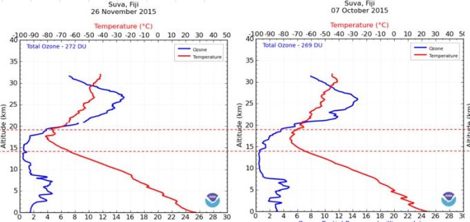
Suva is the capital city of Fiji located at 18° south latitude on the margin of a very large area of high surface pressure that spreads eastward to South America. We see that total column ozone values at this latitude are comparable to the Antarctic in summer and there is a marked deficit in ozone between about 7 and 17 km in elevation, not greatly different to the circumstance in the Antarctic in October.There is a similar ‘hole’ to that in Antarctica but the Suva hole is invariable. If air of this nature travels to Antarctica (and it does) it will be seen to be NOx rich and ozone poor.
An interesting variation in the ozone content of the air occurs in the troposphere. It is clearly related to the shape of the temperature profile. As ozone dissipates from these stratified layers into the air above and below it will affect cloud cover. In October and November average rainfall in Suva is in excess of 200 mm per month. Surface temperature varies between 23 and 26°C across the year peaking in February. As the air warms it has the capacity to absorb more moisture. In a warming regime clouds will disappear resulting in a warmer surface on land or increased absorption of energy by the sea. We call this weather on daily time scales, seasonal variation on inter-annual time scales and climate change on longer time scales and its all entirely natural in origin.
The tropopause is well marked and much elevated at all times of the year. The temperature profile above about 18 km in elevation indicates a strong response to the presence of ozone that is only possible in relatively still air. The temperature of the air increases at elevations above 27km (20hPa) despite the falling away of ozone partial pressure indicating a strong contribution from ionising short wave radiation from the sun in the very exposed latitudes close to the equator. Above 20 hPa there is only 2% of the atmosphere to intercept short wave energy from the sun.

3. Pago Pago
Pago Pago is situated at 14° south latitude in the south west Pacific. The ozone regime is very similar to that at Suva. Notice the temperature response to the presence of 5-6ppm ozone quite close to the surface on 9th December. As Gordon Dobson observed, it is not uncommon to find parcels of very dry air from the stratosphere in places where they are least expected.


4. Huntsville Alabama.
Huntsville Alabama experiences a great deal of diversity in the nature of the air masses, the ozone content of the air, the ozone profile, the speed and ozone content of the wind at different elevations and therefore the height of the tropopause. Note that on the 12th March there is a minor temperature response despite the presence of 10 ppm ozone at 13-15 km of elevation. This suggests that an influx of relatively ozone rich air from higher cooler latitudes is responsible for the low temperature, apparently a relatively frequent phenomenon. On the 2nd March at 10 km in elevation we have 10 ppm ozone and no temperature response at all.
5 Trinidad Head, Humbolt County, Northern California 40° north latitude


Trinidad Head is much subject to a rising and falling tropopause as the ozone content of the air changes with the origin of the travelling air masses. The stated total column ozone value for the 20th January of 99999 Dobson Units illustrates the magnitude of the error that is possible when using ‘climatological tables’ to infer total column ozone when the helium balloon carrying the ozonesonde bursts at a low altitude.
CONCLUSIONS
- Ozone maps surface pressure. The primary driver of change in surface pressure globally is the variation in the ozone content of the air between the surface and 50 hPa.
- The variability in the ozone content of the air manifests in both the troposphere and the stratosphere in the main between between about 7 km in elevation through to 20 km in elevation (350 hPa to 50 hPa).
- The vigorous lateral circulation of the air at and above 250 hPa is a prime driver of the ozone content of the air at particular locations on a day to day basis. The lateral movement of the air in the upper troposphere-lower stratosphere is associated with changes in surface pressure and weather on day to day time scales.
- Ozone at 4 ppm in the lower troposphere can drive an increase in the temperature of the air. This will affect cloud cover and in a regime of changing ozone partial pressure that will drive change in climate. This appears to be the mechanism behind the observed relationship between geopotential height and the temperature at the surface of the planet.
- Change in the ozone content of the air is responsible for change in the weather on day to day intervals and the climate on longer time scales. As Gordon Dobson discovered in the 1920’s Total Column ozone maps surface atmospheric pressure. Unfortunately ‘climate science’ went on a mathematical picnic in the 1960’s and has yet to return to the task of coming to grips with the nature of weather and climate, as it is observed and as it evolves. Dobson was first and foremost an observer and secondly an enormously resourceful inventor of instruments to gather the data necessary to describe the nature of the atmosphere and its modes of change. He left little in the way of written work but his ‘Exploring the Atmosphere’ of 1963 is seminal.
- The atmosphere has a history that is indissolubly linked to the evolution of surface atmospheric pressure at 60-70° south latitude.
LINKS TO EARLIER CHAPTERS
Reality
How the Earth warms and cools in the short term….200 years or so…the De Vries cycle
Links to chapters 1-23
https://reality348.wordpress.com/2015/12/20/how-do-we-know-things/
https://reality348.wordpress.com/2015/12/24/2-assessing-climate-change-in-your-own-habitat/
https://reality348.wordpress.com/2015/12/29/3-how-the-earth-warms-and-cools-naturally/
https://reality348.wordpress.com/2016/01/09/4-the-geography-of-the-stratosphere-mk2/
https://reality348.wordpress.com/2016/01/11/5-the-enigma-of-thecold-corepolar-cyclone/
https://reality348.wordpress.com/2016/01/13/6-the-poverty-of-climatology/
https://reality348.wordpress.com/2016/01/15/8-volatility-in-temperature/
https://reality348.wordpress.com/2016/01/24/9-mankind-in-a-cloud-of-confusion/
https://reality348.wordpress.com/2016/03/10/15-science-versus-propaganda/
https://reality348.wordpress.com/2016/03/18/16-on-being-relevant-and-logical/
https://reality348.wordpress.com/2016/03/26/17-why-is-the-stratosphere-warm/
https://reality348.wordpress.com/2016/04/03/18-the-ozone-pulse-surface-pressure-and-wind/
https://reality348.wordpress.com/2016/04/24/21-the-weather-sphere-powering-the-winds/
https://reality348.wordpress.com/2016/05/04/22-antarctica-the-circulation-of-the-air-in-august/

Hi Erl, chapter 18, PHYSICS OF THE ATMOSPHERE AND CLIMATE MURRY L. SALBY Macquarie University, is an interedting read. Should be right up your street with respect to ozone and nitroxides. I am redaing it between your material. Cheers, Macha.
LikeLike
Looking forward to some informed comment Macha.
LikeLike
Reblogged this on CraigM350.
LikeLike
RE: conclusion1″ The primary driver of surface pressure globally is the variation in the ozone content of the air between the surface and 50 hPa.”.
Do you mean to say this or “The primary driver of CHANGES in surface pressure globally is….”
because surely gravity is THE primary driver of pressure at the surface.
LikeLike
Macha, You are right. I will change it.
LikeLike
I need to think through conclusion 4 too. I thought ozone is very soluble in water, so the cause effect relationship, and presence/absence gets tricky at near surface alitiudes ie where clouds form. The ppmv of ozone would drop in presence of water. I can then see NOx dominate ozone destructive effect at high altitudes, just before UV finishes it off.
LikeLike
Theoretically yes. But practically, when I observe the distribution of tracers of O3 and H2O at 50hPa they lie together. Similarly, across the area occupied by the chain of polar cyclones around Antarctica there is both ozone and NOx. I guess NOx is a catalyst and is not used up so that is understandable. I can’t understand the conjunction with water but its definitely there.
I agree The ppmv of ozone would drop in presence of water. But perhaps it takes time. Perhaps its the fact that the water may be in the form of ice? Perhaps ozone can co-exist with the gaseous form but not with the liquid form? Over to you.
LikeLike
Regards to ozone and water mixes, I do recall somewhere that humidity and dew points are really really low at the poles. This should acount for higher probability for ozone to survive. And yes, catalysts are preserved hence ability to react several times over.
LikeLike
Cant help but pass on this link. I think it might help generate some alternative ways to put concept into wotds…….also some strong chemistry re: OZONE, temperature, velocity, pressures, etc. https://chiefio.wordpress.com/2012/12/12/tropopause-rules/
I see it as largely complimetary.
LikeLike
And my final contribution….This paper: http://www.atmos-chem-phys.net/11/3937/2011/acp-11-3937-2011.pdf. a paper you might like as much as I do because its observational not just desk jockey work.
LikeLike
Hi Macha. The concept of the Brewer Dobson circulation is this and I quote from the paper: The tropical upwelling into the stratosphere, defined as the mass flux through the 100 hPa isobar, increased after the year 2000 (Randel et al., 2006). Consequently, extratropical downwelling through this pressure surface should have increased similarly due to mass conservation. Thus, the ozone mixing ratios on pressure surfaces should have increased in the extratropical lower stratosphere by the intensified downwelling in the same manner as ozone has decreased in the tropics by the intensified upwelling (Randel et al., 2006).
Lots of talk, no conclusion. It appears that they see ‘wave breaking’ as a big influence and suggest that we don’t really understand its influence. Despite its apparent durability I don’t think the Brewer Dobson circulation idea actually applies. It could not, given the lack of variability in the partial pressure of ozone at the equator and the marked variability that we see in the region of the poles and the mid latitudes, account for the variations observed.
Personally, I see the rate of influx of mesospheric air over the poles as the major driver of ozone partial pressure and from Antarctica in particular. That is a function of surface pressure over the pole. The talk of ‘waves’ of various descriptions whether Planetary, Gravitations, Rossby, and ‘wave breaking’ I find deeply dissatisfying.
Now, I haven’t looked at Randall and the notion that intensified upwelling in the tropics could cause an increase in the ozone content of the air in the tropical stratosphere and I find that notion so unphysical that I wont bother myself to look.
LikeLike
Macha says: May 27, 2016 at 8:30 pm
“And my final contribution….This paper: http://www.atmos-chem-phys.net/11/3937/2011/acp-11-3937-2011.pdf. a paper you might like as much as I do because its observational not just desk jockey work.”
Macha,
Thank you for your contribution! Most informative!
Erl,
Macha seems young, with formal education in chemistry, little experience, but most eager to learn more of what is. You seem to have much experience in what you do best! Wine-making!
As farmer (mechanical, oxen, replaced by better stuff), valuable experience!
Electrical, stick welder, used to glue back together the metal parts of broken machinery, just to break again! Valuable experience! Engineering must do ‘close enough for government work’;. Nothing is ‘pearfect’!
Macha has learned ‘chemistry’ inherent in wine-making but remains the most pedantic of all the hard sciences. In Chemistry any dyslexia in the string of chemical letters describing your fine ‘wine’ can lead to product ‘deadly’ on even the slightest sip. Please encourage Macha to learn more of what is! Learning is the GOAL!! Knowing is much overrated!
LikeLike
Hi Erl,
JoNova did a piece involving (Emmert, Lean, Picone, 2010) “Record-low
thermospheric density during the 2008 solar minimum”, GRL 37, L12102.
Because Emmert was implying a Co2 connection, the conversation didn’t
go where I hoped it would.
How hot is that hot layer in the thermosphere? And how does the thermosphere
play into the release of heat?
LikeLike
TL. Mango. Have you a link to the Jo Nova discussion? Neither Google or her site search facility are bringing it up.
I had a look at the Emmert paper. The tipping point reference amazed me? I couldn’t see how he got to that conclusion.
There is a subsequent paper by SOLOMON ET AL.: CAUSES OF LOW THERMOSPHERIC DENSITY
Click to access SolomonJGR2011.pdf
After much careful guesswork a 30% reduction in thermospheric density is attributed in the main to the reduction in the intensity of extreme ultraviolet that is inferred rather than measured. A possible contribution of increased CO2 emitting infrared of 3% is inferred but as to why that should occur escapes me. I thought CO2, like ozone exchanged its energy of excitation with surrounding molecules instantly. The gap in the infrared spectrum measured by satellites that is used to calculate the distribution and partial pressure of ozone represents straight depletion.
Their conclusion: . In these simulations, CO2 and geomagnetic activity play small but significant roles, and the primary cause of the low temperatures and densities remains the unusually low levels of solar EUV irradiance (27% of the 30% reduction in density at 400km elevation).
At 10hPa or 30km you are already above 99% of the mass of the atmosphere. In my not so humble opinion there is no impediment to the release of heat anywhere in the atmosphere. There are always plenty of other molecules to exchange heat with, plenty of scope for convection. Lots of space between the molecules for radiant energy to escape. Wind plays a part in the energy transfer process always tending to create more space where space is needed. A free atmosphere is not an insulator…….if you find some of that anywhere let me know. There are places where I could use it!
The CO2 argument is pure fantasy. I know it to be so because the atmosphere tells us so as I relate here: https://reality348.wordpress.com/2016/03/26/17-why-is-the-stratosphere-warm/ Its to do with the temperature of the surface and the tropopause in winter where at the surface the air is coolest in winter while at the tropopause the air is coolest in summer.
LikeLike
Thanks for your consideration…very gentlemanly of you all.
I am still reading. It seems to me the key to ozone interactions is not the actual oxygen to ozone, or reverse, reaction energy perse, its the remnant solar UV frequency. The intensity of this energy that’s able to reach the earth in absence of ozone and in particlar, the ocean, is where the substational heat (capacity) is held and thermalised. Ozone generation and destruction is vast and hence explains why imbalances can be seen in only hours. The lack of ozone in troposhere is primarily due to lack of UV penetration at right frequency to be created from oxygen. What is seen in the atmospheric temperature and ozone concentrations is a product rather than a cause. The root cause is solar (UV) and water…… Ps. No doubt i need to work on converting thoughts into words.
LikeLike
I think your site will get more traffic…..http://notrickszone.com/2016/05/28/solar-deniers-face-harsh-times-flurry-of-new-studies-cern-show-suns-massive-impact-on-global-climate/
. “Solar variability can influence surface climate, for example by affecting the mid-to-high-latitude surface pressure gradient associated with the North Atlantic Oscillation1. One key mechanism behind such an influence is the absorption of solar ultraviolet (UV) radiation by ozone in the tropical stratosphere, a process that modifies temperature and wind patterns and hence wave propagation and atmospheric circulation”
Macha
LikeLike
Hi Erl,
The JoNova piece is:
“Another climate model paper in Nature misses . . . . .”
Third discussion down from the home page.
I agree with you the Co2 argument is fantasy.
And your work involving stratospheric cooling and ozone is solid.
But, what really peaked my interest was the connection between
thermospheric density and solar activity.
The earth’s dynamo is regulated by specific motions of the
sun/earth/moon system. A weakening of the earth’s magnetic field
would allow more UV to enter the thermosphere. So it isn’t just
a matter of the solar wind hitting the magnetic field, but also how
much we let in. There must be a direct connection between the earth’s
magnetic field strength and thermospheric density. If charged particles
are involved in stratospheric cooling, they must first pass through the
thermosphere.
LikeLike
TL Mango,
As I understand it from reading stuff like this EUV at a wave length of up to 124 nm is responsible for the ionization of the atmosphere above 80km in elevation. I quote: The ionosphere is what we term a weak plasma, as only one percent of the neutral atoms in the upper atmosphere are ionised. Traces of ionisation exist from about 80 km to 1000 km in altitude, with the peak ionisation occurring around an altitude of 300 km. The maximum ionisation can vary from about 1010 to 1013 electrons per cubic metre.
Ionospheric ionisation is controlled by extreme ultraviolet and soft x-ray flux emitted by the Sun. The lower regions of the ionosphere show almost exclusive solar control in that the ionisation at any time is proportional to some function of the solar zenith angle. The volume of atmospheric gases that are involved in the ionization process is less than the 1% of the mass of the atmosphere that is above the 10hPa pressure level.
The inflation of the atmosphere due to ionization gives rise to atmospheric drag experienced by satellites at an elevation of 400km. The reduction in solar activity over the last thirty years has enabled satellites to travel closer to the Earth and orbit for longer. EUV varies much more than total solar irradiance.
The presence of the moon does not modulate UV activity from the sun. The solar wind impacts the ionosphere but it will not affect cooling rates in either the ionosphere or the stratosphere.
My personal opinion is that the Earth’s temperature is not modulated by so called ‘cooling rates’. I think ‘cooling rates’ would be only a factor in static air, air that is trapped within some form of ‘insulation’ and that does not occur in the atmosphere. Never.
LikeLike
The increase in the speed of the solar wind caused a stronger jet stream in the polar vortex and enlargement of the ozone hole.


Erl, in the mesosphere radiates of infrared N2O.
LikeLike
RE the solar wind and Geomagnetic activity. All the studies I have seen indicate a warming of the winter stratosphere under the influence of increased Ga involving a fall in surface pressure at the pole, a rise in the mid latitudes and a warming of the winter stratosphere. So, I suggest the zonal wind reduces in velocity under GA activity and the stratosphere cools as the mesospheric tongue shrinks away.
LikeLike
The temperature increase of the polar circle in the winter may be associated with an increase of N2O as a result of a stronger ionization.
LikeLike
This is the theory. Increase in NOx in the inflow of mesospheric air should reduce the ozone content of the air in the mesospheric tongue and the stratosphere generally via mixing processes across the vortex, reduce the pressure differential across the vortex, slow polar cyclone activity, enable a return of atmospheric mass to high latitudes thereby increasing surface pressure and result in a further fall of ozone partial pressure as the mesospheric tongue penetrates further.
The history of the southern stratosphere since 1948 has involved a reduced intake of mesospheric air as surface pressure has fallen away over Antarctica enabling ozone partial pressure to increase. This produced a peak in the temperature at 10hPa over Antarctica in 1978 and temperature has gradually fallen away since that time.
LikeLike
In winter, more specifically N20 can increase the infrared radiation, since ozone decreases the polar circle. Ionization must concern just O3 and O2
(the breakdown of particles to atoms).
LikeLike
Ren, Not sure I understand your point.
Is the ionization that is a product of cosmic rays capable of directly giving rise to ozone? Reducing ozone? There is a theory that says Cosmic Radiation breaks down CFCs. However I don’t think that path for ozone depletion is responsible for the Antarctic ozone hole.
LikeLike
Such a large increase in ionization in the winter can cause strong galactic radiation, accordance with the field lines Earth’s magnetic field. Then suddenly it appears more free oxygen atoms.
LikeLike
So, you are saying that ozone is broken down directly by cosmic radiation? Is there evidence?
LikeLike
Erl look at the situation at an altitude of over 20 km.
LikeLike
A lot of ozone is accumulating at 1 hPa with vortex interference developing in the last few days. http://macc.aeronomie.be/4_NRT_products/5_Browse_plots/1_Snapshot_maps/index.php?src=MACC_o-suite&l=TC Look at a plot of the ozone over the last 9 days. Yes, would need to check same time same place across recent years to see this in perspective.
LikeLike
Ren, Thanks for the reminder. The ozone pattern varies with elevation. Lots of ozone build up at 1hPa http://www.cpc.ncep.noaa.gov/products/stratosphere/strat_a_f/gif_files/gfs_o3mr_01_sh_f00.png and even better seen at http://macc.aeronomie.be/4_NRT_products/5_Browse_plots/1_Snapshot_maps/index.php?src=MACC_o-suite&l=TC
I am very surprised to see new ozone data for levels below 100 hPa. Somebody is perhaps waking up to the action that drives the jet stream at 250hPa. http://www.cpc.ncep.noaa.gov/products/stratosphere/strat_a_f/gif_files/gfs_o3mr_250_sh_f00.png
And down to 400hPa. This is new to me and a big surprise. We see ozone at 400 hpa in the regions where mid latitude high pressure cells form up. Hey, this is impressive. Now, if they could get the resolution that we see the Europeans manage to achieve we might learn something.
LikeLike
Abstract. The Specified Dynamics version of the Whole Atmosphere Community Climate Model (SD-WACCM) and the Goddard Space Flight Center two-dimensional (GSFC 2-D) models are used to investigate the effect of galactic cosmic rays (GCRs) on the atmosphere over the 1960–2010 time period. The Nowcast of Atmospheric Ionizing Radiation for Aviation Safety (NAIRAS) computation of the GCR-caused ionization rates are used in these simulations. GCR-caused maximum NOx increases of 4–15 % are computed in the Southern polar troposphere with associated ozone increases of 1–2 %. NOx increases of ∼ 1–6 % are calculated for the lower stratosphere with associated ozone decreases of 0.2–1 %. The primary impact of GCRs on ozone was due to their production of NOx. The impact of GCRs varies with the atmospheric chlorine loading, sulfate aerosol loading, and solar cycle variation. Because of the interference between the NOx and ClOx ozone loss cycles (e.g., the ClO + NO2+ M → ClONO2+ M reaction) and the change in the importance of ClOx in the ozone budget, GCRs cause larger atmospheric impacts with less chlorine loading. GCRs also cause larger atmospheric impacts with less sulfate aerosol loading and for years closer to solar minimum. GCR-caused decreases of annual average global total ozone (AAGTO) were computed to be 0.2 % or less with GCR-caused column ozone increases between 1000 and 100 hPa of 0.08 % or less and GCR-caused column ozone decreases between 100 and 1 hPa of 0.23 % or less. Although these computed ozone impacts are small, GCRs provide a natural influence on ozone and need to be quantified over long time periods. This result serves as a lower limit because of the use of the ionization model NAIRAS/HZETRN which underestimates the ion production by neglecting electromagnetic and muon branches of the cosmic ray induced cascade. This will be corrected in future works.
http://www.atmos-chem-phys.net/16/5853/2016/
LikeLike
The total NOy produced per year from GCRs was compared
with that from other sources. GSFC 2-D model calculations
show that N2O oxidation (N2O + O(1D)→NO + NO) produce
43.5–55.7 GigaMoles of NOy with the vast majority
(greater than 90 %) produced in the stratosphere. GCRs were
computed to produce 3.1–6.4 GigaMoles of NOy , with 40–
50 % of that produced in the stratosphere. Thus, GCRs can
be responsible for as much as 14 % of the total NOy production,
however on average, GCRs produce about 3–6 % of
stratospheric NOy in any given year. This is somewhat less
than that found by Vitt and Jackman (1996), who computed
that GCRs were responsible for 9–12 % of the total stratospheric
NOy produced per year. The Vitt and Jackman (1996)
computations used ion pair production rates from a parameterization
based on yearly averaged sunspot number from
Nicolet (1975), which are generally larger than those GCRcaused
ion pair production rates computed with the more recent NAIRAS model used in the present study (discussed in
Sect. 2).
Click to access Jackman_acp-16-5853-2016.pdf
LikeLike
Ren, It appears that there are lots of competing entities produced by ionization processes according to calculations. What we need is systematic observation rather than modelling and guesswork by mathematics.
LikeLike
Primary ionization of main atmospheric constituents by GCR.
The efficiency of the direct ionization of N2, O2 and O3
– calculated by the Maxwell–Boltzmann distribution (see eq. M1), are given on Table1. It can beseen that despite the lower ionization potential of O2
(compare reactions (1) and(3)), the efficiency of the N2
ionization is 2.88 times greater because of its highernumber density (remember that the ratio of nitrogen to oxygen molecules in the lower atmosphere is N2/O2≈3.7).
Through reassessment of the efficiency of main atmospheric constituents’ ionization by GCR and the ion-molecular reactions between the most abundant ionsand neutrals, we have shown an existence of an autocatalytic cycle for continuous O3
production in the lower stratosphere and upper troposphere (near the level of maximal absorption of GCR, known as Pfotzer maximum). The quantity of O3
,produced by the positive ion chemistry, has the same order of magnitude as themid-latitude steady-state ozone profile. This is an indication that the lowermostozone profile could be substantially distorted by the highly energetic particles.
http://www.academia.edu/3190232/An_autocatalytic_cycle_for_ozone_production_in_the_lower_stratosphere_initiated_by_galactic_cosmic_rays
LikeLike
Thanks Ren that’s useful stuff.
LikeLike
Ren, a very interesting paper. If they are right it brings in a whole new dynamic in terms of reasons for the ozone peak in high latitudes in winter. But there is more: GCR deposition into the lower atmosphere depends on the temperature of the air in the polar cap region. So, higher ozone content and a warmer stratosphere is subject to a multiplier effect tending to generate more ozone. Lower surface pressure at the pole reduces the intake of mesospheric air, ozone proliferates, polar cyclone activity accelerates further lowering surface pressure and the GCR activity cuts in to accelerate the production of ozone as the polar cap warms. Just as well gravity is there to constrain the process.
LikeLike
Erl, GCR grow and see what happens in the lower stratosphere in the north.
LikeLike
Erl, GCR systematically growing to the level of 2006.
http://cosmicrays.oulu.fi/webform/query.cgi?startday=01&startmonth=05&startyear=2001&starttime=00%3A00&endday=01&endmonth=06&endyear=2016&endtime=00%3A00&resolution=Automatic+choice&picture=on
LikeLike
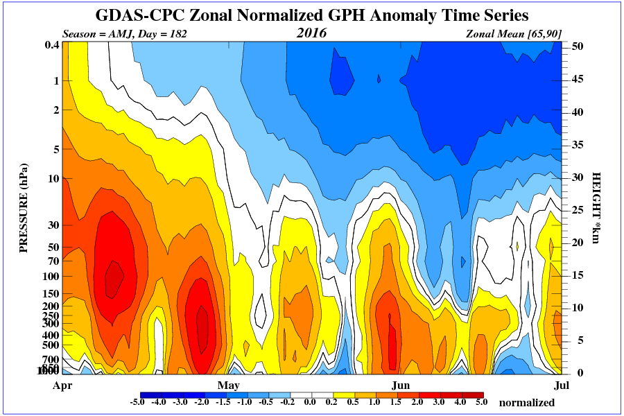
Ren, As I understand it the Z anomaly is represents the difference in the temperature of the Arctic stratosphere over recent months by comparison with climatology. So, lower geopotential height in the upper stratosphere reflects a cooler upper stratosphere than normal. It should directly reflect anomalies in the AO index not the index itself. That cooler air at the top of the column is due to higher polar pressure and increased zonal (West to East) wind and an increased proportion of cold mesospheric air in the mix. Shows that the AO index is moving to the negative. I just want to make sure we agree on what we are looking at so check with me the following:
We are here:http://www.cpc.ncep.noaa.gov/products/stratosphere/strat-trop/
This shows the actual temperature:http://www.cpc.ncep.noaa.gov/products/stratosphere/strat-trop/gif_files/time_pres_TEMP_MEAN_AMJ_NH_2016.png
This shows the temperature anomaly: http://www.cpc.ncep.noaa.gov/products/stratosphere/strat-trop/gif_files/time_pres_TEMP_ANOM_AMJ_NH_2016.png
This shows the Zonal wind slowing down as the stratopshere warms towards summer: http://www.cpc.ncep.noaa.gov/products/stratosphere/strat-trop/gif_files/time_pres_UGRD_MEAN_AMJ_NH_2016.png
This shows the Zonal wind departure from normal showing speeding up in May: http://www.cpc.ncep.noaa.gov/products/stratosphere/strat-trop/gif_files/time_pres_UGRD_ANOM_AMJ_NH_2016.png
This (Z anomaly) shows the ANOMALY in GPH indicating reduced GPH as the upper stratosphere shows cooling below normal: http://www.cpc.ncep.noaa.gov/products/stratosphere/strat-trop/gif_files/time_pres_HGT_ANOM_AMJ_NH_2016.png That is in conformity with increased zonal wind being in more mesospheric air and an anomalously cool stratosphere.
This reflects the reduced incidence of ozone derived convection that takes warm air up to 10hPa and higher or in other words the stratospheric warmings: http://www.cpc.ncep.noaa.gov/products/stratosphere/strat-trop/gif_files/time_pres_WAVE1_MEAN_AMJ_NH_2016.png
Do we agree on this interpretation?
This shows the recent elevation of warm air into the region of the polar cap in the southern hemisphere://www.cpc.ncep.noaa.gov/products/stratosphere/strat-trop/gif_files/time_pres_HGT_ANOM_AMJ_SH_2016.png
That warm air shows up in high ozone partial pressure over the Indian Ocean that is generated east of South Africa and over New Zealand. Can be seen here: http://macc.aeronomie.be/4_NRT_products/5_Browse_plots/1_Snapshot_maps/index.php?src=MACC_o-suite&l=TC make sure you bring up southern hemisphere at 1hPa for ozone centred on 2016-06-01
The GCR are permitted to do their work as the stratosphere over the pole warms. That’s why the flow of muons gives us a record of stratospheric warmings. Now, if that Russian author is correct GCR by virtue of their ionization of the air over the polar cap result in more ozone as the upper atmosphere warms. If the upper atmosphere cools GCR are excluded and less ozone is created tending to reinforce the cooling. Finally, the amount of GCR over the pole increases as the solar wind falls away so its greatest near solar minimum. But the solar wind as reflected in the aa index does not vary strictly with sunspot activity or the flux in EUV radiation. So GCR peaked after the last solar minimum by about a year. Do you agree with all of this?
LikeLike
When the vortex
is strong (~1980-2010) meridional processes in the troposphere intensify and GCR increase is accompanied
by an enhancement both of cyclonic activity at middle latitudes and anticyclone formation at polar ones.
When the vortex is weak (~1950-1980) the meridional circulation weakens and GCR effects change the sign.
Thus, the ~60-year variation of the amplitude and sign of SA/GCR effects on troposphere pressure seem to
be closely related to the vortex state and the corresponding changes in the evolution of the large-scale
atmospheric circulation. It should also be stressed that at the present time the vortex seems to change its state
(see Fig.2c, d), so we could expect a reversal of those correlations which were observed between dynamic
processes in the lower atmosphere and SA/GCR characteristics during the last thirty years.
Fig.3b shows the height dependences of the characteristics of the Arctic air mass where the vortex is
formed calculated for January 2005 on the base of NCEP/NCAR reanalysis data, as well as that of ion
production rate caused by GCR in free air at polar latitudes. We can see that the temperature in the vortex
center decreases with the increase of height and reaches its minimum at the levels 30-50 hPa (20-25 km).
The temperature gradients at the vortex edges increase with height in the stratosphere starting from the level
150 hPa, their maximum being observed at the levels 50-10 hPa (20-30 km). In the troposphere temperature
gradients are maximal near surface corresponding to Arctic fronts separating the Arctic air from warmer air
of middle latitudes. Thus, the vortex is most pronounced at the 50-30 hPa levels where the minimum of
stratospheric temperatures and the maximum of temperature gradients at its edges are observed. We can see
that the highest values of ion production rate due to GCR are observed in the lower part of the vortex (10-15
km) where temperature gradients start increasing. On the other hand, the 11-year modulation of GCR fluxes
is strongest at the heights 20-25 km [Bazilevskaya et al., 2008] where the vortex is most pronounced. Hence,
the vortex location seems to be favorable for the mechanisms of solar activity influence on the atmosphere
circulation involving GCR variations. It is also favorable for the mechanisms involving solar UV variations,
as at these heights (15-25 km) in the polar stratosphere the maximum ozone content is observed.
Click to access Veretenenko_%20et_all_Geocosmos2012proceedings.pdf
LikeLike
In my opinion, due to a decrease UV (low sunspot activity) GCR role in the production of ozone (and N2O) will increase. Because circulation will a more depend on the Earth’s magnetic field.
LikeLike
This will be reflected in the distribution of temperature (due to the drop of UV average temperature could drop).

LikeLike
During the summer waves over the polar circles are less visible. Perhaps due the lack of the polar vortex.
LikeLike
Hi Ren,
Sorry about the lack of a reply for such a long time. First I went away then I had to write in order to get some things clear and be able to answer questions properly. One of them is this question of ‘waves’. I consider that the so called waves are due to the build up of ozone outside the core of mesospheric air situated over the polar cap. Ozone accumulates in particular places. The land masses promote high surface pressure in winter due to their coldness. The sea is warm and it promotes low surface pressure. Ozone is drawn into the low pressure circulations creating the cyclones that morph into a laminar flow at Jet Stream altitudes that constitutes the lower margin of the stratospheric ‘vortex’ But, the presence of a relatively stationary zone of low surface pressure over the ocean that constantly draws in ozone rich air is responsible for two phenomena that dissipate the consequent overload of ozone. The first of these is the tongues or traces of ozone rich air that are left behind and spread out towards low latitudes and the second is episodic convection of warmer air to the top of the column. At 1 hPa the mushrooming of ozone partial pressure occurs on a ten day cycle that relates to the time it takes for a mid latitude anticyclone to pass a particular point non the Earth’s surface. I illustrate this in Chapter 25 just posted. The maps also give an excellent view of the polar vortex that is ozone deficient at 1 hPa.
LikeLike
Erl look as the temperature in the lower stratosphere depends on the magnetic activity (UV) sun.

Lower Stratosphere:http://vortex.nsstc.uah.edu/data/msu/v6.0beta/tls/uahncdc_ls_6.0beta5.txt
http://www.drroyspencer.com/2016/06/uah-global-temperature-update-for-may-2016-0-55-deg-c/
LikeLike
Its now four days in a row without sunspots. “The Svensmark solar mechanism leads to more intense cosmic rays during weak solar activity, thus resulting in up to a 100-times more powerful cloud-formation affect in the troposphere, as confirmed by the Swiss research facility CERN:”
so much water available to be split into ozone by UV / cosmic radiation, reaching an less magnetically well-shield earth, so at that high altitude of cloud formation would be felt as cooling at ground level, yes? might this produce higher temperature gradient / lapse rate which leads on to bigger pressure differences and higher winds. Chaos in moving air masses from equator to poles (earth is a spinning Sphere so fastest and hottest in middle) leads to any manner of vortexes, and subsequent rough weather events. Will be looking into latest volcanic activity to find interferences to ozone, Br, Cl, NOx levels too.
LikeLike