28 MISREPRESENTING THE TRUTH

It is an article of faith in climate science that the temperature of the stratosphere is due to the impact of short wave radiation. This is incorrect. In fact the temperature of the stratosphere is due to the interception of long wave radiation from the Earth by ozone. It is another article of faith that the circulation of the air is driven from the tropics. This is also incorrect.

The temperature of the atmosphere  reflects many forces at work but the most important of these so far as the circulation of the air is concerned is ozone. The ozonosphere can be considered to extend from the surface of the planet through to the mesopause. The shape of the ozonosphere is a product of  a number of forces:

• The interaction of short wave solar radiation with the atmosphere that supplies oxygen in atomic form to combine with O2 to form O3.  This occurs in the mesosphere down to about 60 km in elevation and also it seems at the poles where cosmic rays ionise the atmosphere allowing the formation of ozone.
• The tropical atmosphere below about 40  kilometres in elevation exhibits an increase in its ozone content in daylight hours and may be considered a relatively safe zone where ozone can accumulate in trace amounts.
• Relief from the pressure of ionisation at low sun angles. Ozone is  ionised by  UVB and shorter  wave lengths that are used up in the process. Because the atmospheric path is long very little ultraviolet B reaches the polar regions to destroy ozone and none at all during the period of the polar night.
• The lower profile of the stratosphere is sculpted by the erosive activity of NOx  that is influential in establishing the height of the tropopause and in the process determines the elevation where the maximum in ozone partial pressure occurs.
• At the poles the intake of mesospheric air varies on all time scales and regulates ozone partial pressure accordingly.

The ozone content of the air and the height of the troposphere so established are influential in determining surface pressure and therefore the flow of the air, in fact the location and intensity of the planetary winds that regulate the equator to pole temperature gradient and the extent and location of cloud cover that limits the incidence of solar radiation at the surface.

To examine the profile of the stratosphere at all latitudes would be a worthy but onerous task that I will leave to others.  But it is instructive to study the temperature of the atmosphere in a  particular latitude band to try and discern the forces at work because they are different according to hemisphere and latitude. I look in particular at the temperature of the air in the latitude band 30-40° south at selected levels  starting  at the planets skin, then 2 metres above the surface, at 700 hPa,  at 500 hPa where half the atmosphere is below and half  above, 300 hPa where something quite strange begins to happen,  at 200 hPa and 100 hPa  where paradoxically the air is warmer in winter than in summer. Then we look at the temperature of the air at 30 Mb and at 10 Mb therefore spanning 99% of the depth of the atmosphere. This site is the starting point:  http://www.esrl.noaa.gov/psd/map/time_plot/

A SURVEY OF THE ATMOSPHERIC PROFILE AT 30-40° SOUTH LATITUDE.

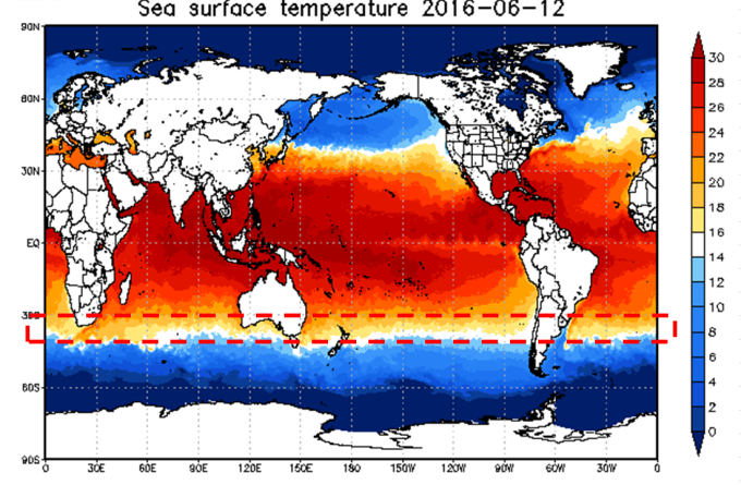
The map above shows the latitude band under investigation. It is mostly sea.

The hovmoller diagram below shows the average temperature at the surface across the 30-40° south latitude band as it evolves  in the interval of the single year 2014. There is nothing special about this year. Any year would do.

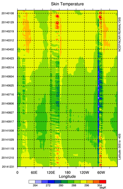
The skin temperature exhibits a pattern of summer warming influenced by the location of the land masses of South Africa, Australia-New Zealand and South America. There is marked warming of the Pacific Ocean from November through to June. There are southward moving warm currents on the west of the ocean basins and up welling of cold waters on the east of the basins particularly to the west of South America. Also seen is the remarkably episodic pattern in the cooling of the Australian continent in winter that relates to an intermittent flow of cold air that traverses the continent from north west to south east. The Pacific maintains a zone of relative warmth to the east of the Australian continent perhaps by virtue of the relative width of the ocean and the strength of the southerly trending circulation of warm waters from the tropics.The land masses warm strongly in summer.Notice the strong cooling of the Indian Ocean to the west of Australia in winter-spring that tends to promote the formation of a sticky zone of high atmospheric pressure. In contrast the warmth of the Pacific in the vicinity of New Zealand creates s sticky zone of low surface pressure.

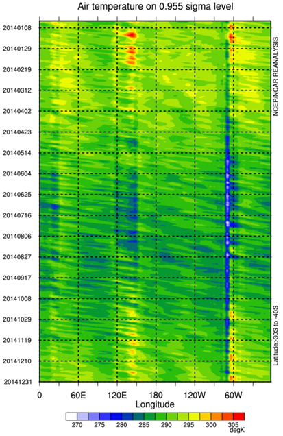
The proposition advanced in climate science is that the temperature of the air predominantly reflects the temperature of the skin. Above we see that even at 2 metres of elevation this is not the case. Already  warming and cooling is intermittent within a season by comparison with skin temperature. The scale necessary to span the variation in the temperature of the skin spans 48°C. The scale required at 2 metres is only 4o° C. The land masses cool the air in winter while air over the sea remains warmer. Texture in the temperature data is produced  by moving air bodies that originate in the north west (called the westerlies) that locate towards the south east at a later date reflecting the fact that the atmosphere rotates faster than the Earth itself and propagates towards the south east carrying tropical warmth to higher latitudes but in an intermittent fashion.The warm air is also wet and arrives with cloud. The presence of cloud can be erroneously considered to be the source of the warmth via back radiation whereas the air is actually warm because of its origin. In fact any particular location on the Earths surface will be warm or cool according to the origin of the air. If the air changes in either its speed or direction this alters the equator to pole temperature gradient. 

The ultimate  fate of the air in these latitudes is to be drawn into a low pressure cyclone located at 50-70° south latitude. We see that the pattern made by the north westerlies is more defined in winter and spring than in summer and autumn. Autumn is a pleasant time of the year in some of the windiest latitudes on the planet. By latitude as we move southwards from the thirties we have the Roaring Forties, the Furious Fifties and the Screaming Sixties. In winter the Thirties assume some of the character of the Forties.

Warmer air manifests in shorter strings with less persistence probably because it is rising and leaving the cold air at the surface in long remnant streamers. Cold air, locally chilled as it travels over cold water pools into the valleys of Andes mountains in winter.  There is a clearer definition of summer and winter in the temperature at 2 metres than in skin temperature.  We see that the atmosphere heavily influences near surface air temperature regardless of the status of skin temperature. Temperature is not simply a function of the angle of the sun. Cloud cover plays a part in determining local air temperature. Not shown is precipitation rates and relative humidity that exhibit the same north west to south east streaming. The Pacific sector to the East of 150° east longitude is wetter than the Indian ocean sector. The temperature pattern indicates a slowing or a blocking of the the atmospheric flow in the Western Pacific when compared to the other oceans. We have blobs rather than streaks and reduced contrast.

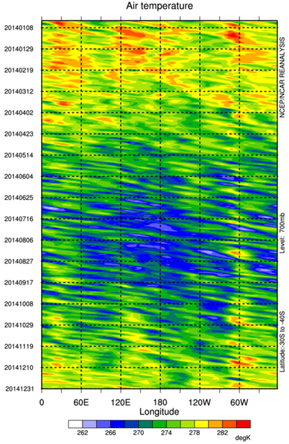
At 700 Mb (above) there is a a thicker, broader structure in the pattern of temperature variability in summer and thinner more linear elements in winter. This indicates a faster air flow in winter. In summer and autumn the air is relatively still. There is more seasonal definition at 700 mb than at 2 metre elevation emphasising that the movement of the atmosphere is influential in  creating seasonal contrasts. It is the movement of the atmosphere that defines the equator to pole temperature gradient. If the wind blows alternately from a warm place and then a cold place we call it an oscillation, such as the Arctic Oscillation or the Antarctic Oscillation.

There is a much stronger graininess  in temperature at 700 Mb than at the surface emphasising the dependence of surface conditions on the state of the atmosphere as it varies on short time scales. The degree of graininess is different according to longitude with the appearance of persistent linear elements in winter that propagate south eastwards more strongly in some parts than others.

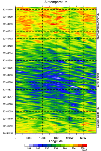
At  500 Mb (above) there is a similar pattern to that at 700 Mb but the winter season is shorter.  In the vicinity of Africa the air is warmer  across the year . This likely represents a consistent flow of warm tropical air southwards in that vicinity.

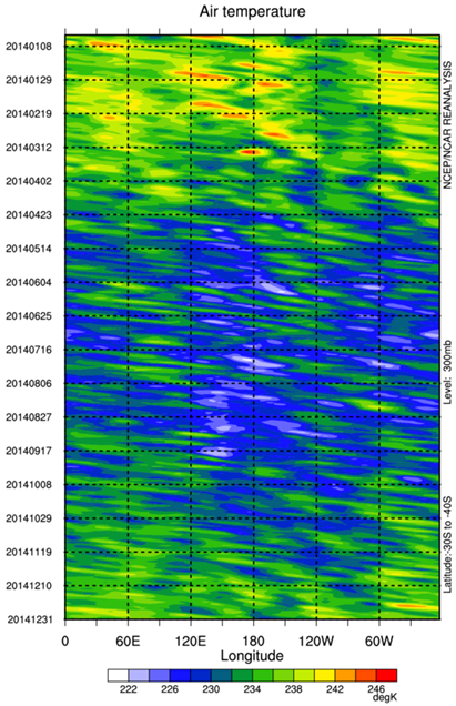
At 300 Mb there appears to be a marked extension of the winter season and reduced contrast between the seasons.

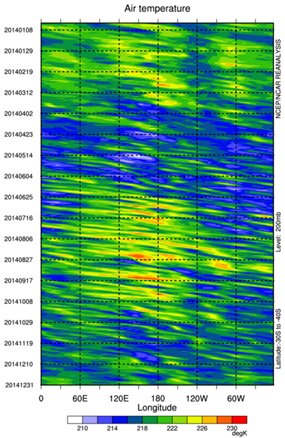
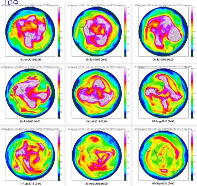
At 200 Mb (above) we see that the months June to October are  warmer than the summer months.  In particular this is the case between longitudes 60° East and 120° West. This relates to the pattern of the increase in atmospheric ozone in winter. We have entered a realm in the upper troposphere where the temperature of the air is markedly influenced by the presence of ozone. There  can be no active photolysis of  any atmospheric gas at the 200 mb to  drive the warming of the air. Rather, heating is due to  energy gain from infrared radiation that is emanating from the Earth itself. The ozone molecule absorbs at 9-10 um. This is a phenomenon unrecognised and unremarked in climate science even though ozone is recognised as a ‘greenhouse gas? The 200 mb pressure level is the altitude where jet streams manifest. Each small yellow-orange streak in the diagram above represents a stream of ozone warmed air that is rapidly ascending. There is a strong linearity and persistence in the patterns in this diagram. The pattern is quite different to that  seen at lower altitudes. The difference  relates to the marked change in density differentials between different air masses. Notice the concentration of warming  between longitudes 120-180°  East. due to the tendency of ozone to accumulate in low pressure cells in the southern ocean to the south of Australia and New Zealand. This is  verified in the diagrams below that represent ozone at 1 hPa on the 16th day of the month, each diagram a month apart.

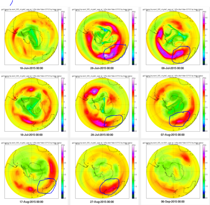
Above we have a polar stereographic view of Antarctica at the 1 hPa pressure level. These diagrams show the manner of the descent of ozone deficient mesospheric air over the pole and also the episodic tendency for ozone to accumulate over the Southern Ocean south of Australia and New Zealand at longitude 120 to 180° east of the Greenwich meridian. This tendency is reflected in the hovmoller diagrams both above and below. The heating process due to the increase in ozone partial pressure in winter  delivers an even stronger contrast at the 100 Mb pressure level. In fact the 100 Mb pressure level is where the movement of the bulk of the atmosphere is determined. The temperature of the air and its movement has little to do with surface conditions and a lot to do with the ozone content of the atmosphere that increases strongly in winter.

The diagram above shows air temperature at 100 mb. Winter is warmer than summer at 100 hPa due to ozone heating of the air. The air is warmest in the Australia New Zealand sector due to the tendency for ozone to proliferate over the warm waters of the western Pacific Ocean that tend to promote the formation of zones of low surface pressure.

Above we see the distribution of ozone at 100 hPa over the southern hemisphere in winter. At this elevation the atmosphere shows the texture that would might expect at the interface of two different fluids moving at a slightly different rate but in the same anticlockwise direction. Tracers of ozone rich air emanate from nodes rich in ozone and are left behind in air that moves less rapidly. The nodes of ozone rich air tend to form in the lee of the continents where the waters are warmer and in particular in the Australian, New Zealand western Pacific sector.

The anticlockwise circulation of the air moves faster than the Earth itself and faster in the polar regions than at the equator. This gives rise to some very interesting questions: Is the force that causes the Earth to rotate on its axis also responsible for the faster rotating atmosphere, a disengaged fluid element that is free to reflect the forces of the interplanetary environment acting on the atmosphere? Are these forces responsible for the minute variations that are observed in the Length of the Day that are seen to be related to changes in climate as we measure it at the surface of the Earth? Is this rotation of the Earth and its atmosphere driven by the same sort of force that drives an electric motor.  Does the atmosphere simply exhibit an amplified variation of the length of day type that could be  measured in terms of the speed and direction of the high altitude winds. Does the rotation of the air speed up and slow down as the electromagnetic field changes under the influence of the sun and the solar wind?

Notice the generalised depletion of ozone that starts in August. This is due to the activity of NOx reaching the pole as surface pressure rises, the flow of mesospheric air is cut off and the final warming begins. In springtime as atmospheric pressure falls over Antarctica the stratosphere over the pole warms, the circulation of the air slows and by December it actually reverses its rotation at the 10 Mb level.

In particular we should be interested in whether the zonal wind slows as the stratosphere heats, not only on the annual scale, but also on the synoptic scale of days and weeks. If it does, perhaps the atmosphere is responding to the electromagnetic environment of which it is part.

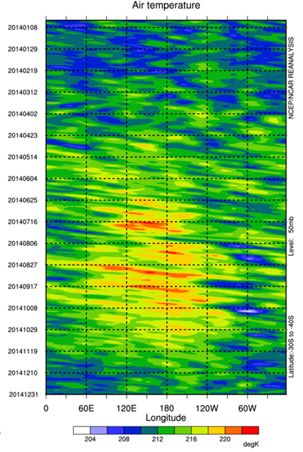
At 50 hPa (above) the pattern of ozone accumulation in the Australian New Zealand sector is more clearly defined. The pattern is less episodic, more linear and  persistent. In fact the movement of the air even at 30° -40° south begins to reflect the linearity and the stop-go nature of the high altitude zonal wind that reaches its apogee in the structure of the polar vortex.Notice the difference in linearity between summer and winter. Notice the extension of winter warming until November that is the transition month between winter and summer conditions at this latitude. We are here looking at part of the driver for surface conditions in the southern hemisphere and indeed globally on all time scales.In a later chapter we will see that November is the ‘snap to attention’ month when the dominant role of driving the ozone content of the air is passed over short time intervals is passed, baton like, to the Arctic.

There is one other thing worth noticing. Its actually extremely important because it confounds what we read in Climate Science texts. The 50 hPa pressure level  is in the lower stratosphere at an elevation of 20 km. The stratosphere is supposedly stratified, non convective and irrelevant so far as surface weather is concerned. In fact the stratosphere in winter is a very active part of the atmosphere in terms of air temperature, density and wind. Inspect the scale on this diagram. The range required to represent the data at 50 Mb is 22°C. At 100 hPa the range is 30°C. At 500 hPa the range required is 28°C, at 700 hPa 26°C and at 2 metres 40° C. What does that tell us about the forces responsible for the movement of the atmosphere? The atmosphere is a medium that tends to minimise temperature differences in the horizontal plane. The range at 100 Mb, though flattened by winter warming, indicates that the forces that are involved in generating air temperature and density contrasts aloft are more influential in driving the movement of the air than the forces that are active at the surface. The range required at 100 Mb  is diminished by the reversal of the temperature relationship between summer and winter, a range reducing phenomenon that  acts to conceal rather than reveal the forces at work . Perhaps a  superior proxy for the  strength of the disparities in density at 100 Mb is wind strength. Wind strength is least at the surface and increases with elevation peaking at Jet Stream altitudes. The inevitable conclusion is that the movement of the bulk of the atmosphere at 30-40° south latitude is driven at the  100 hPa pressure level or thereabouts by differences in the partial pressure of ozone as it effects atmospheric temperature and density.

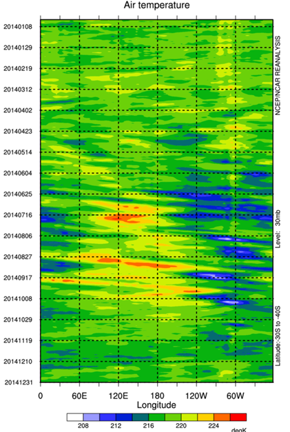
Above we see air temperature at the 30 Mb pressure level.The difference between summer and winter is greatly reduced. The range of variation is still greater in winter than summer. Only in winter do we see the characteristic north west to south east flow of the winter stratosphere. The patterns that are generated indicate strong  variations in the temperature and density of the air related to the changing composition of the air itself. However, it appears that this is a zone where air tends to either descend or ascend (blobs rather than streaks) rather than travel laterally except in the winter where the circulation is more typical of that which prevails all the way to the surface.

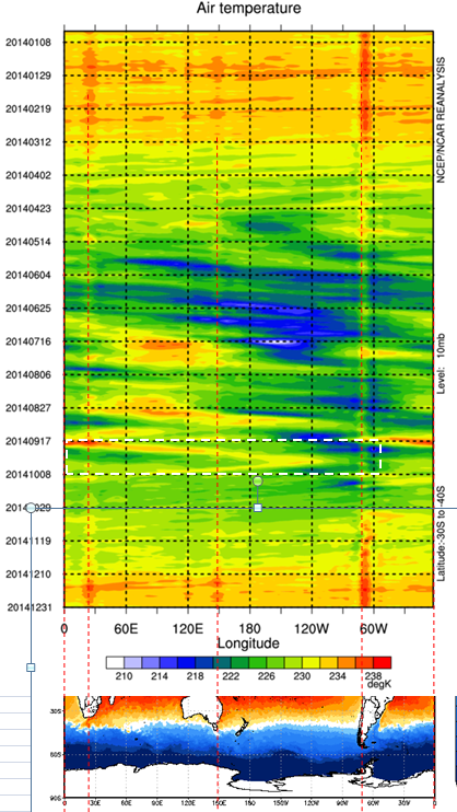
At the 10 hPa pressure level (above) the air is comparatively still. Only the strongest elements of the ozone driven winter circulation show up. Notice the south west to north east drift in summer as ozone rich air travels towards the zone of high surface pressure in the mid latitudes. The flow is north west to south east in winter. Here the temperature of the air relates to surface temperature in a manner that is not evident between 700 mb and 30 mb. The winter is cold and the summer warm as we would expect it to be. The land masses are especially warm. So, most surprisingly we see the signature of surface temperature at 10 hPa,  an elevation where 99% of the mass of the atmosphere lies beneath.The warmth of the air plainly relates to the interception of infrared radiation by ozone. Because the air is relatively still at this altitude the pattern of long wave emission from the surface shows up. If short wave radiation from the sun were a big influence on the ozone content and the temperature of the air at this altitude this pattern would be obliterated in daylight hours. We cant tell from this diagram whether this happens or not.

There could be no better demonstration of the response of the stratosphere to the infrared radiation emitted by the Earth than this phenomenon. We see it because the air is relatively still. The temperature of the ozonosphere that stretches from the surface through to the mesopause  is set, not by ionising  radiation from the sun but radiation from the Earth itself. There is little variation in the ozone content of the air or its temperature at 10 mb that we can link to the tenfold variation in EUV across the solar cycle. Plainly, it is incorrect to maintain that the temperature of the stratosphere is a function of ionisation by short wave radiation from the sun. This statement, to be found universally in climate texts and the works of the UNIPCC and in Wikipedia does not square with observation.

We must look for other modes of causation for the potent variations in the ozone content of the air in winter than variations in the quantum of short wave energy from the sun. Indeed, only one percent of the air above 80 km in elevation, the zone called the ‘ionosphere’, is actually ionised. This zone contains less than 1% of the mass of the atmosphere. There is no problem in supply and no problem in persistence of ozone below the 10 Mb pressure level. The ozone content of the atmosphere is relatively invariable and seems to be assured, but not so at the poles in winter where we see big variations in ozone partial pressure from year to year.

If we look for zones where atmospheric dynamics involve a dilution of the ozone content of the air that can account for the paucity of ozone over the polar caps, the marked variations in the ozone content of the air from week to week and year to year and the relative paucity of ozone in the southern hemisphere in general we need look no further than the polar vortex in the winter season.

THE ZONAL WIND

The zonal wind is that which is measured as rate of travel a along a line of latitude and is called the ‘u’ wind while the meridional wind is that measured along a line of longitude and is designated as the ‘v’ wind. At a point on the Earths surface a wind can be described in terms of both u and v. It is weak in both u and v it is probably descending or ascending.

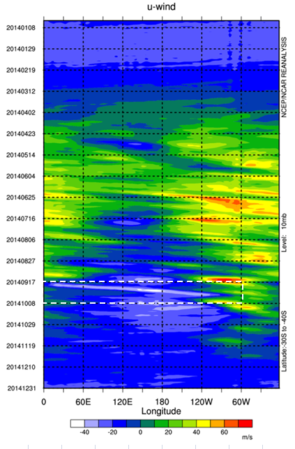
If we inspect the last several diagrams they all indicate a strong stream of warm air travelling around the globe in a south easterly direction after 2014-09-17. The timing of this warming air flow is associated with a collapse of the ‘u’ component, a symptom of warming over the polar cap associated with an increase in the ozone content of the air  that is further associated with a collapse of surface pressure over the pole. This is a  taste of that which happens in the transition between winter and summer. It is also closely associated with the appearance of the ozone hole over Antarctica when NOx rich air of tropical origin circles in to occupy the entirety of the polar cap between 100 hPa and 50 hPa.

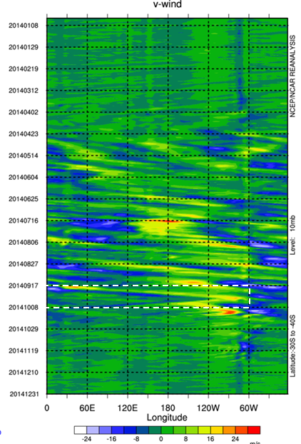
As we see above the ‘v’ component of the wind at 10 Mb is seasonally the mirror image of the ‘u’ wind. The meridional component falls away as the zonal wind component increases and vice versa.This is true on a seasonal as well as an episodic short term basis.

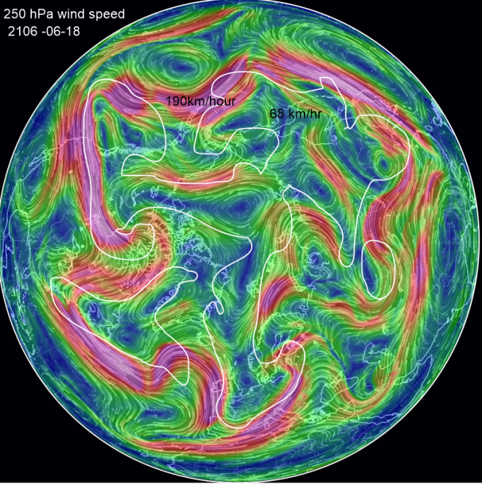
It is apparent that the movements of the atmosphere are tied to the partial pressure of ozone in the stratosphere. This is readily apparent when we study the movement of the air over the polar cap at 200 Mb as represented below. The first diagram shows the distribution of ozone over the Arctic on the 18th June 2016 as shown  here. The second diagram shows the temperature of the air and its circulation over the Arctic on the 18th June 2016 as shown here.  The third diagram simply shows the speed of the wind and locates the jet streams in relation to the distribution of ozone.

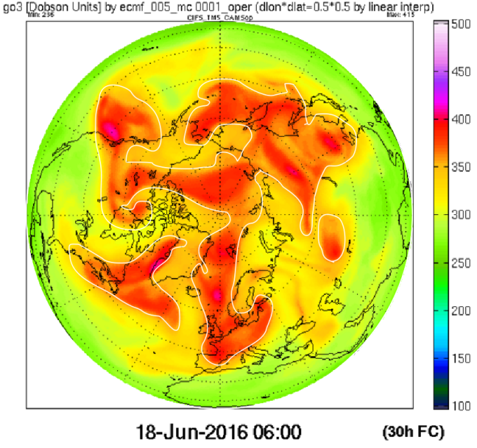
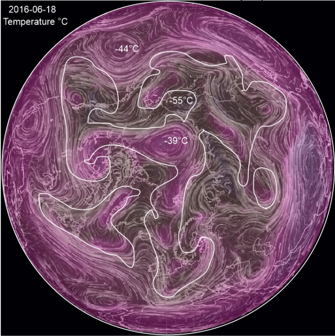
There is a core of cold air over the Antarctic within which pockets of ozone rich air are almost 20° C warmer. The conjunction of the two gives rise to the jet streams as we see below.

CONCLUSION

• The movement of the air is intimately associated with contrasts in ozone density.  Speed of movement  is greatest at jet stream altitudes where contrasts in air temperature and density are most extreme.
• Change in the intensity of the zonal wind that is associated with warming and cooling at the surface occur in response to the impact of ozone on atmospheric motions. In the northern hemisphere this phenomenon can be expressed in terms of the Arctic Oscillation, the North Atlantic Oscillation or the Northern Annular mode.In the southern hemisphere we talk of the Southern Annular mode. These are all recognised as prime modes of climate variation on annual and inter-decadal time scales. Climate science has no rationale for any of them and is unable to differentiate between climate change due to these entirely natural phenomena and that supposedly due to the activities of man.
• Climate change is associated with change in the ozone content of the air that drives the intensity of polar cyclone activity, shifts in atmospheric mass, change in the zonal wind and the equator to pole temperature gradient.
• Winter is the season where weather variability is greatest and this is clearly associated with change in the ozone content of the air. This is backed up by the observation that across all latitudes the month of greatest variability in surface temperature is either January or July as described here.
• The circulation of the atmosphere is not driven from the equator but from the winter pole. There is evidence that the ozone content of the air at the poles depends upon solar activity via several different modes.

Unless we can separate out and properly account for the change in climate that is due to the fluctuating ozone content of the air we are in no position to quantify the change that many attribute to the works of man.  Green activists  are clearly ‘jumping the gun’. When we come to look at the manner in which the climate changes according to latitude it will be plain that all change, I repeat ALL change, is very likely attributable to natural modes of causation rather than the works of man and we will be able to say, ‘hand on heart’, or on a ‘stack of bibles’ and ‘with a very high level of confidence’ that we are speaking the truth.